free site design templates
Mobirise

This tutorial teaches the basic methods to define problems, perform calculations and to get related results.  Pictures shown here are from calculations with version 3.0, but of course the tutorial can be used without any change in version 3.1, 3.2 and 3.3 too. Tutorials 3.1, 3.2 and 3.3 below are related to the new sorts of magnets and methods, which have been introduced in those versions.

Circumferentially magnetized multipolar magnet with six poles 

This tutorial shows the basic handling of the software as well as its basic characteristics. The problem which shall be teated here consists of a cylinder made of six homogenous segments of anisotropic ferrite, having a remanence induction of 0.40T each. The example below and similar problems ca be treated by use of the demo version of PS-PERMAG and for sure by the full versions 3.0 or 3.1. The additional features of both versions which are not shown here can also be learned easily by use of their extensive help system. The treatment of the new two pole sensormagnets of version 3.1 with enhanced geometric details can be studied in Tutorial 3.1

After starting PS-PERMAG a 3D model of an illustrative permanent magnet shows up on the screen. To define the above described magnet please click on the M symbol at the top symbol bar. M stands for circumferentially magnetized multipolar cylinders with homogenous magnetization in each pole. This opens an input dialog for the data input, see picture below. Here the basic data of the magnet have to be put in. Background for defining a cylindrical magnet is always a cylindrical coordinate system. This means e.g. that at half the axial length of the magnet there is always z=0. At zero angle phi=0 there always starts an outward oriented pole.

Mobirise
After you press OK the respective new 3D model shows up on the screen including the defined results path, see the picture below this text. You can zoom in or out of the model by using your mouse central wheel. By a left mouse click and simultaneous mouse movement one can turn the model around its x- or y-coordinate axis. By a right click together with a mouse movement the model can be moved horizontally or vertically. Simultaneous left click and use of the shift key on your keyboard will let you turn the assembly around the z-axis. A general method to increase or decrease the screen contents may also be the use of the + or - button in the second symbol bar. By pressing one of them them beside the 3D magnet model also all other contents of the screen can be changed by size. With the help of the neighbored SO symbol respective zoom factors for texts and diagrams can be stored as defaults for any new calculations. By this it is possible to adjust the software to the users screen resolution. The coordinate system symbol you can switch on and off by the respective button in the second symbol bar. Please push now the GO-button to start the field calculations. After a few seconds they should be completed. The progress will be shown by a respective progress bar. Please push then the button to show a diagram for the results of the radial field component as indicated in the picture below by the arrow. The button there shows the letters r and x. The three neighbored buttons to the right stand for the other two field components as well as for the absolute field value.
Mobirise
Now look onto your first results. These are the values of the radial field component as a function of the circular angle. Instead of using the full angular range it can be cut to a defined interval. To change the diagram please click on the respective button on the left side of the second row of symbols, see the picture below. By this an input dialog will open to let you change the start and stop angle. In case you want to return from the field diagram back to the 3D magnet model, please click the respective button in the right half of the second symbol bar. Right beside this button (here in grey) are three option buttons for the 3D model (Hide/Show coordinate triangle, Transparent magnet model, Default position).
Mobirise
The fields can also be presented as numerical listings, which can be opened by clicking on the respective bright gray buttons in the first symbol bar. The first of these buttons opens the listing of the radial component when cylindrical result coordinates are used. For systems needing cartesian coordinates this button shows the x-component. Generally for cylindrical magnets by default a cylindrical coordinate system for the resulting components is applied. But for all kinds of magnets also cartesian coordinates can be chosen for the output. By clicking the button with the two doted lines in the options bar (second symbol bar) one can change the total number of values which PS-PERMAG computes on a chosen path. To finalize such change the computation has to be repeated by using the GO button. 
Mobirise
Additional calculations based on the single field components are e.g. Fourier series expansions. In case you would like to have an overview over the approximation of e.g. the radial field by such series, please click in the third bar (evaluation bar) and there on the first of the gray symbols in the last quad. Then the original curve together with its Fourier approximations up to specified grades are graphed. Below this is shown for the first two poles after having constricted the geometric diagram angle to 180deg. Which and how many grades are chosen for graphical depiction can be determined by clicking the first button of the second symbol bar. A listing of all numerical coefficients of the Fourier series can be shown for each single field component by clicking on the respective button with letter c in the third symbol bar, like shown below by the respective arrow. In addition the distribution of different wave orders can also be shown graphically by clicking the respective button in the second last quad of the third row of symbols.
Mobirise
Another sort of evaluations are field angles which are of importance e.g. in sensor technology. In the evaluation bar (third row) a click on the respective button of the second triplet reveals these angles graphically. Below the angle of the field projection in the r-phi plane is shown. The buttons of the first triplet provide the respective numerical listings of these angles. All angles are defined between -180deg and +180deg. Graph colours can be chosen generally in the options bar as being shown by the respective button and its dialog mask below.
Mobirise
For field evaluation beside circular paths for all kinds of magnets also straight lined paths can be defined. In addition all results on all sorts of paths can be shown in cylindrical as well as in cartesian coordinates. In the picture below the respective buttons for the change of path geometry and also for the choice of result coordinates are marked by respective arrows. By choosing the button for defining a magnet after having switched to a linear path, an input dialog as shown below will open. To display the 3D model as shown below again the switching button in the second symbol bar is to be used. The linear path is displayed by a green line. In the case below the linear path shall run 1mm above the center of the first pole, starting at a radius of 12mm and ending at 24mm. Due to the input dialog linear paths are always defined by their cartesian coordinates of start and end point locations. Because the center of the first pole is located at 30° here, and as the axial length of the magnet is defined as hm=6mm, the following coordinates for the start point location have to be put in: x=12*cos(30)=10.392, y=12*sin(30)=6.0,z=hm/2+1=4.0. The respective figures for the end of the linear path are: x=24*cos(30)=20.785, y=24*sin(30)=12.0, z=hm/2+1=4.0. After finishing the input dialog the computation has to be started by use of the Go button.
Mobirise
In the next screenshot we show the result of the x component of the field after a problem definition on a linear path like in the picture above. The result coordinate system has been switched to cartesian coordinates here. Because we have a straight line path the results are shown as a function of distance.
Mobirise
To close this tutorial some additional features should be mentioned: In the first symbol bar a dialog can be chosen to put in your own text of a description of the analysis. Beside the common binary storage of the analysis, which does not only include all primary and secondary results but also the most current user adjustments of the software, in addition an ASCII file of the field values by using the “txt” button can be written. Another button of importance is the red button close to the “Go” symbol, which lets you stop a current computation. The options bar, in addition to its already mentioned features, also provides features like changing the accuracy of computation or entering and storing your personal data, which will then always be shown on the detailed printouts of PS-PERMAG. The size of the screen view can be adjusted to your demands using the + and - buttons. Additionally a specific button in the options bar opens a dialog which lets you adjust subjects like the thickness of letters or diagram curves or the visibility of diagram grids. Three sorts of option buttons handle the storage and recover of the user adjustments of the software. Not to forget: All features, which are usable by the above described buttons, can also be used by clicking on their respective menu commands, which are included in the main menu bar on top of the program window. Additional features of the software can be learned easily by use of its extensive help system.

Tutorial 3.1

Learn here to handle the new features of version 3.1. New two pole sensor magnets with ledges and depressions

Input of an axially magnetized two pole sensormagnet with depressions and ledges

This tutorial shows the geometry input of the new sorts of two pole sensormagnets with depression and ledges, which have been added in PS-PERMAG version 3.1. The basic use of PS-PERMAG can be studied in Tutorial 3.0.

The following treats a two pole, axially magnetized sensormagnet. The geometry input of the other two new sorts of magnets, i.e. two pole diametrical and two pole axial-lateral, has to be done by the same way. First there has to be defined a basic cylinder. Depressions and ledges will be subtracted from this basic cylinder by up to four additional help volumes.

Mobirise
A depression on the magnets top face can be defined by the input of radius and height of help volume V1, which will be subtracted from the basic cylinder, see next picture.
Mobirise
If a ledge on the outside of the top face is needed, help volume V2 can be used. The radius r2 here stands for the radial depth of the ledge beginning at the outside of the basic cylinder, see the next picture.
Mobirise
If at the bottom face another circular depression is needed this can be modeled with the help of volume V3. See next picture
Mobirise
Finally another ledge can be built also at the bottom face, here with volume V4. The radius again stands for the radial length starting at the outer circumference of the basic cylinder.
Mobirise

Tutorial 3.2

In this tutorial we explain three new features of verion 3.2. These are the rotatable result coordinates, the cuboit-kit system as well as the feature of axial magnetic bearings.

Rotatable Result-Coordinates
In version 3.2 for all sorts of magnets rotatable result coordinates were introduced. With this feature the respective coordinate system can be rotated about its own axes so that new coordinate systems result. Amongst others this is of importance for magnetic sensors. In such systems marginal tolerances  during their assemby or inside the sensorchips of a few 0.01mm can lead to serious lacks of positional accuracy. With the new feature of rotatable coordinate systems the impact of related effects can be studied. In the picture below the tilt of a sensor by 5deg around its cylindrical r-axis is being defined as an example.
Mobirise
Is the sensor by system tolerances 1mm radially remote from the center of rotation, a tilt of the sensor by e.g. those 5deg can lead to serious increases of angular inaccuracy, as can be seen in the listing of field angles below. Here deviations of a few degrees can be observed as shown e.g. at the marked locations..
Mobirise
Cuboid-Kit
By the cuboid-kit assemblies of blocks of different position, size,  different strength and direction of magnetization can be defined. The following picture shows an example with a linear field path.
Mobirise
The following shows an input dialog typical for cuboid-kits. The single blocks are defined by their lower left position in the Cartesian coordinate system. Their extension is defined in x-, y- and z-direction by respective figures for lengths. The direction of magnetization has to be defined by the polar angle with the  z-axis (0 to 180deg) and by the azimuth angle (0 to 360deg).
Mobirise
The following is another example for a cuboit-kit in its 3D view. As for this kind of problems random orientations of magnetization can be defined, directions of magnetization can be vizualized here when setting the 3D view to transparency. The arrows can be switched on and off by the respeictive symbol in the options bar. If it interferes with the 3D symbol of the coordinate system, switch it off with the button left to the transparency button. The arrows show the direction of polarization inside the single cuboids, but do not indicate the strength of magnetization.
Mobirise
Axial Magnetic Bearings
Axial magnetic bearings with arbitrary number of poles can be defined by a new feature of the axially multipolar magnet cylinders. In the input dialog one now has the choice of defining a magnet in front of a soft magnetic plate or of defining the magnet in front of a twin magnet with opposite direction of magnetization. The following screenshot provides a magnetic bearing with four poles per magnet. Here in the input dialog a mutual distance of 5mm was chosen. The software calculates the repulsive force independently from the chosen field path.
Mobirise

Tutorial 3.3

In this tutorial new characteristics of version 3.3 will be elucidated. On one hand this is a continuously changable shape of magnetic polarization within one single sort of magnet. This has been introduced for circumferentially magnetized bow shaped as well as axially magnetized bow shaped cylinder magnets. For multipolar cuboids beside the known alternating rigid magnetization an axially bow shaped magnetization has been added. The latter can also here change its shape in a continuous way. Beside these features, for all magnets the output of two dimensional vector sums in all three spatial planes have been added in version 3.3.  

Laterally bow shaped magnets on circumference with adjustable pole shape

Bow shaped magnetized magnets on circumference  (L-symbol in symbolbar) have by default a sinus shape of polarization with slowly decreasing strength to the inside of the specimen. By this resulting fields do not show any harmonic distortion. On the other hand, for specific applications a more trapezoidal magnetization might be demanded. All kinds of polarization shapes between perfectly sinusoidal and nearly perfectly radial, with an only minor residual transition zone, can now be be realized for this kind of magnet. This can be done by the new so called deformation parameter.  The deformation parameter can be varied between 0 and 1. By that nearly all shapes of magnetization with continuously varying direction within one pole can be modelled. Following picture provides the input dialog of a bow shaped magnetized magnet with the new introduced deformation parameter:

Mobirise

When a deformation parameter > 0 has been given in, a diagram opens which shows the distribution of radial and tangential components of magnetization at the pole surface, also including the polarization's vector sum. By that the grade of deviation from a perfectly sinusoidal polarization is being visualized, together with an impression about the size of transitions zones between poles. For a laterally bow shaped magnetization this is provided always for a whole pole pair. For the four pole magnet above one pole pair covers 180°. In the following picture the deformation parameter has a value of 0.3.

Mobirise
Axially lateral magnetization with adjustable pole shape

Deviations from a perfectly sinusoidal polarization by use of a deformation parameter have been implemented into version 3.3 also for axially lateral cylinder magnets, i.e. magnets with a bow shaped magnetization at one head face. The Following picure reveals the related input dialog for a six-pole magnet, here also with a deformation paramter of 0.3.

Mobirise

Next there is provdided the distribution of polarization components at the magnets pole face as well as the related vector sum. One pole pair here comprises 120°.

Mobirise

The impact on the axial field distribution near the magnets surface can be seen in the following screenshot by some Fourier series aproximations of the signal for a few orders of higher harmonics. The deviation from a perfectly sinusoidal magnetization leads to a harmonic distortion of around 9%, as can be seen on the right side by the respective figure below the listing of Fourier coefficients. 

Mobirise
Multipolar Cuboid with bowed magnetization and adjustable pole shape 

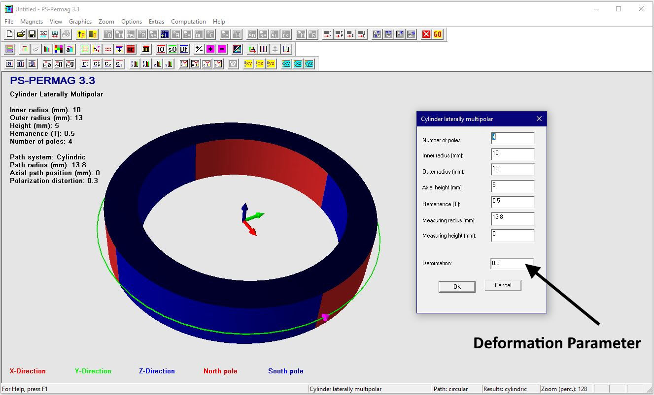
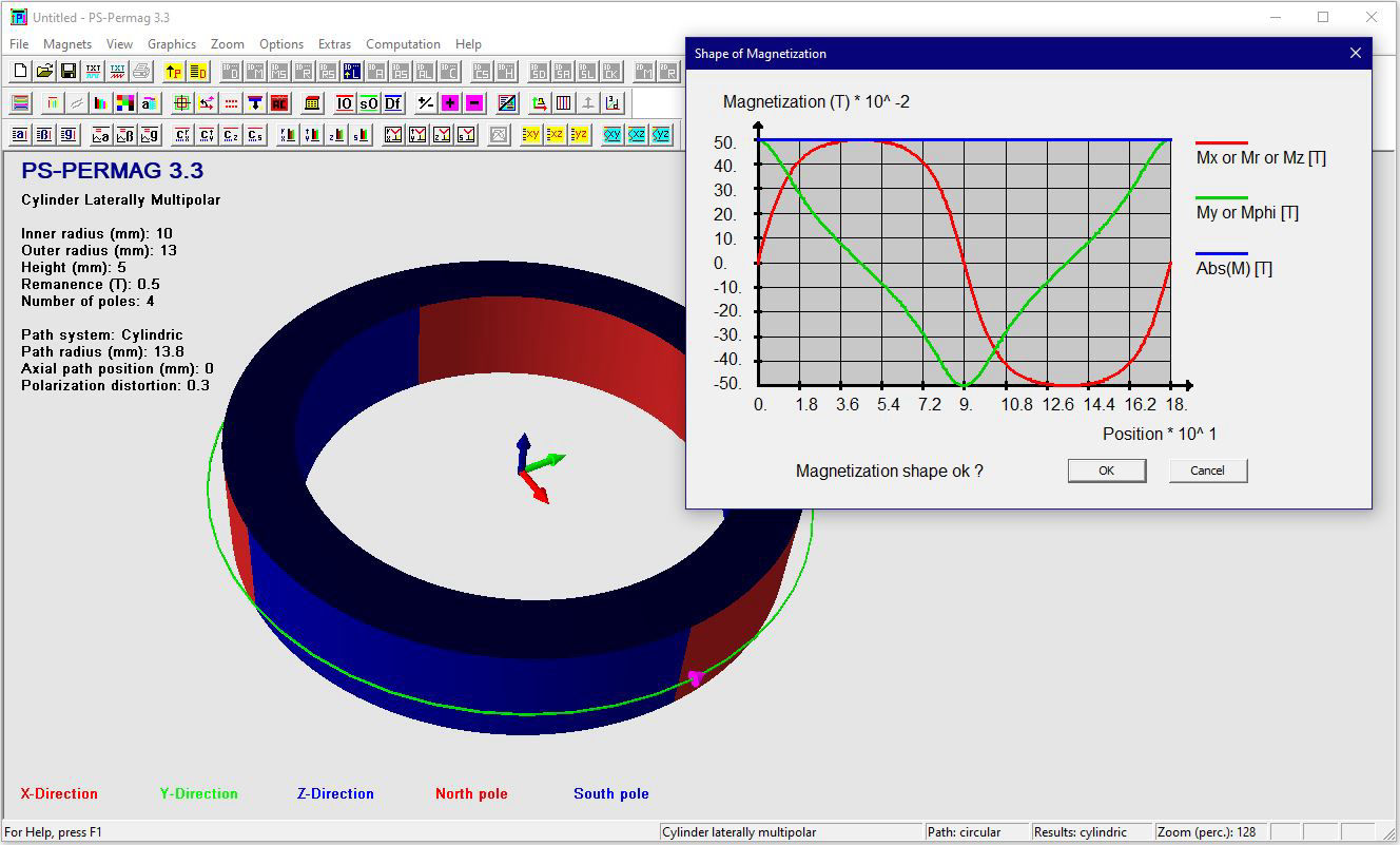
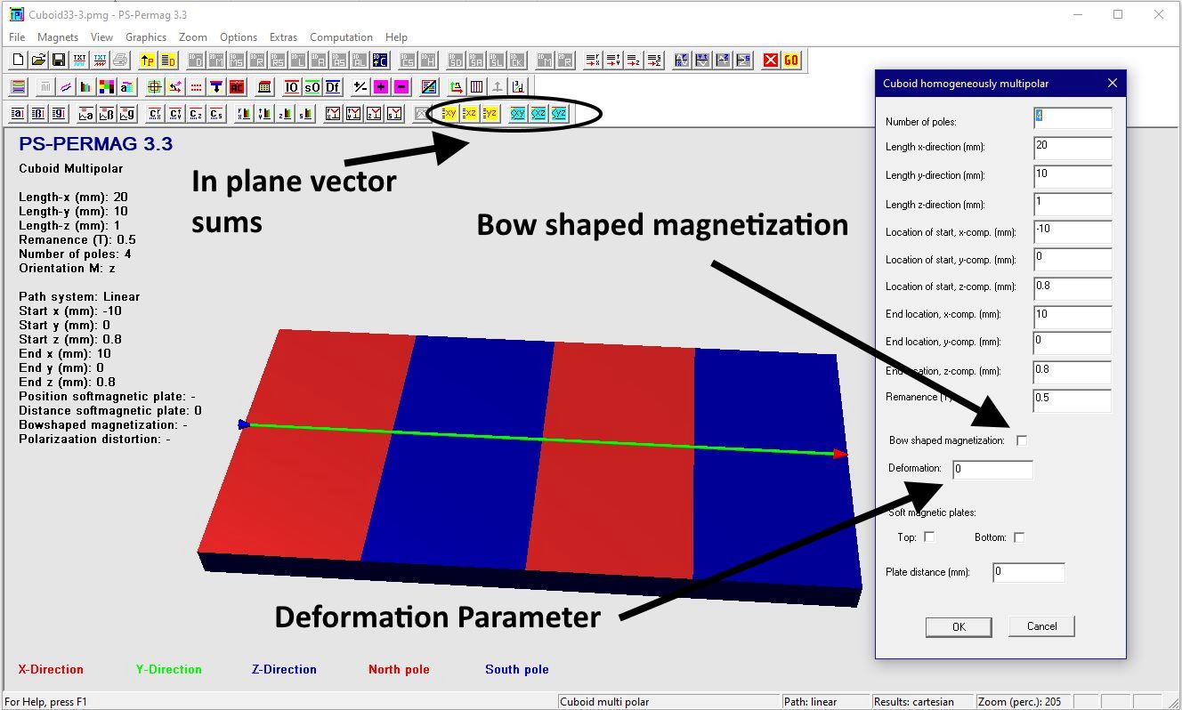
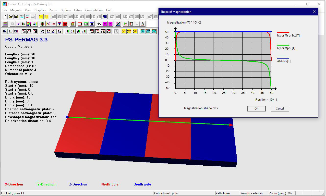
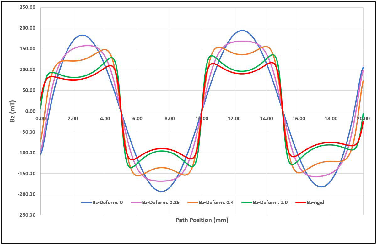
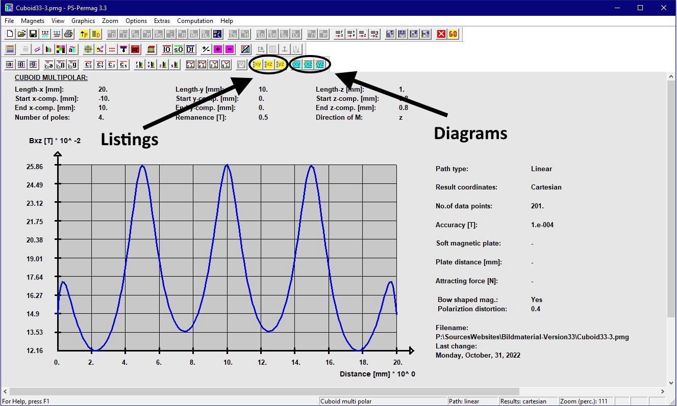
A bow shaped magnetization has been implemented into version 3.3 as a new option for the multipolar cuboid (C-option in symbol bars). The default magnetization for this kind of specimen is still a rigid, alternating magnetization with an uniform direction within the single poles. By marking the respective dialog input as being shown in the following picture, magnetization can be switched to a bow shaped one. If in the input dialog the deformation parameter below is still set to zero, then the polarization will be perfectly sinusoidal, while with other values it is deformed. In case the deformation parameter is 1 a nearly perfect axial magnetization with only minor transition zones to the other poles will me modelled.  When a bow shaped magnetization has been chosen there is always a slow decrease of vector sum of magnetization into the inside of the magnet, as it is mostly the case for a real magnetization process. If the bow shaped magnetization were not marked the deformation parameter would not have an impact on the default rigid magnetization.

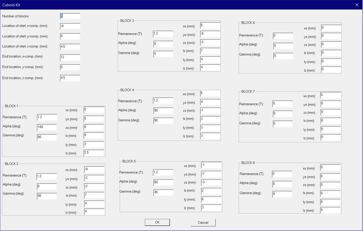
The screenshot below additionally highlights buttons for listings and and diagrams for two- dimensional vector sums, which have been implemented for all kinds of magnets in version 3.3. Those will be treated in the next subchapter.

Mobirise

The next provides the distribution of polarization components when there is the maximum deformation of 1. In the respective diagram for cuboids the polarization shape is always shown along one pole only. In case that the deformation parameter is at its maximum value, the transition zone has only a marginal size as it would take place e.g. after a skillful pulse magnetization process. In case of a perfectly rigid magnatization with perfect uniformity within each single pole, then the option of a bow shaped magnetization should stay unmarked.

Mobirise

The graph below this provides the axial field component near the magnet's surface along the above depicted path after an export of results to a spreadsheet program. Here a bow shaped magnetization was modelled for deformation paramaters of 0.0, 0.25, 0.4 and 1.0. Additionally the result for the rigid polarization has been included.

Mobirise
Two dimensional vector sums in coordinate planes 

The output of two dimensional vector sums is valuable especially for the design of magnetic sensor systems, as here often results in one plane are of interest. For all kinds of field paths these planes can be Cartesian planes (e.g. xy) or cylindric planes (e.g. radial.tangential) acoording to the chosen result coordinate system. The following picture provides for the above defined cuboid system the Bxz- vector sum as a function of the path position, here for a bow shaped magnetization with deformation parameter 0.4. Values always can be displayed as listings as well as graphs. These new features have been implemented to all kinds of magnets that are treated by the PS-PERMAG of the software.

Mobirise